Mixture Models

Latent variables

Latent variables are the random variables whose values are not specified in the observed data. Modeling these latent variables is required to explained the observed data in terms of the unobserved concepts. Since these variables cannot be observed or measured experimentally. Examples:

1. You fit a model to a dataset of scientific papers which tries to identify different topics in the papers, and for each paper, automatically list the topics that it covers. The model wouldn’t know what to call each topic, but you can attach labels manually by inspecting the frequent words in each topic. You then plot how often each topic is discussed in each year.
2. Reduce your energy consumption: you have a device which measures the total energy usage for your house (as a scalar value) for each hour over the course of a month. You want to decompose this signal into a sum of components which you can then try to match to various devices in your house (e.g. computer, refrigerator, washing machine), so that you can figure out which one is wasting the most electricity.

Let \(x\) be observed/visible variables, \(z\) be the latent/hidden variables. We want to model \(p(x, z|\theta)\), so marginalizing over \(z\), we can write \(p(x|\theta) = \sum_z p(x, z|\theta)\) For estimating unknown model parameters \(\theta\), we can compute the Maximum Likelihood Estimate (MLE) on visible variables alone.

Mixture models

When latent variables \(z\) are discrete and observed variables \(x\) are continuous, mixture modeling can be adopted to solve the problem. It aims at maximizing the marginal likelihood of observed variables \(p(x) = \int_{z} p(x,z)\).

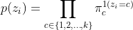
• Type 1: Model assumptions: Discrete categorical latent variables \(z \in \{1,2, ..., k\}\), univariate case: continuous observed variables \(D = \{ x_1, x_2, ..., x_n \}\). The mean \(\mu\) is different and \(\sigma\) is same for each component of Gaussians, mixing weights are known.

Marginal probability \(p(z_i)\):

Gaussian conditional probability:

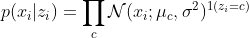
Probability density for one data point \(p(x_i)\):

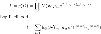
Joint density or likelihood for \(D = \{ x_1, x_2, .., x_n \}\):

Known variables: observed variables \({x}\), mixing weights \(p(z_i=1), p(z_i=2), .., p(z_i=k)\);

Unknown variables: latent variables \(\mu_c, \sigma, c=\{1,..,k\}\)

Method: Expectation-Maximization algorithm

An elegant and powerful approach E-M algorithm, particularly for latent variables, can be used.

E Step:

• fix parameters \(\mu_{a}, \mu_{b}, \mu_{c},\sigma_{a}, \sigma_{b},\sigma_{c}\) and
• compute posterior distribution

M Step:

• fix the posterior distribution

• optimize for \(\mu_{a}, \mu_{b}, \mu_{c}, \sigma_{a}, \sigma_{b},\sigma_{c}\).

MLE estimates are the latent variables $\mu_c, \sigma_c, c={0,1,…,k}$

Using MLE estimates of parameters, following probabilities can be estimated:

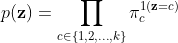
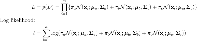
• Type 2: Model assumptions: Discrete categorical latent variables $z \in {1,2, …, k}$, multivariate case: continuous observed variables $\textbf{x}$. The mean $\mu$ and $\sigma$ are different for each component of Gaussians, mixing weights are unknown.

Marginal probability $p(\textbf{z})$:

Conditional probability $p(\textbf{x}|\textbf{z})$:

Joint density or likelihood for $\textbf{x}$:

E-M algorithm can be used.

Known variables: observed variables $\textbf{x}$;

Unkown variables: latent variables $\boldsymbol{\mu}_c, \boldsymbol{\Sigma}_c, c={1,…,k}$, mixing weights $p(\textbf{z}_i=1), p(\textbf{z}_i=2), …, p(\textbf{z}_i=k)$

MLE estimates are the latent variables $\boldsymbol{\mu}_c, \boldsymbol{\Sigma}_c$, mixing weights $\pi_c, c={0,1,…,k}$ Using MLE estimates of parameters, following probabilities can be estimated:

References:

1. Grosse, R., Machine Learning CS 2515